Anaplan Use-Case 9: Aggregating across Time

Often, we find ourselves aggregating data for users. When Time dimension is not the one excluded, we deploy simple aggregation method (SUM/AVG/MIN/MAX/ANY function). However, every now and then, we encounter situations where aggregation involves ditching the Time dimension. How do we deal with such a case?

NOTE: This article is a segment of the Anaplan Use Cases Series. If you haven’t already, I encourage you to go through the introductory blog Why Anaplan Use Cases Series? to understand the background behind this endeavor.

Context

A hypothetical firm Saffire is an agricultural company in India that markets, exports and sells Saffron in USA. The firm grows and harvests four varieties of Saffron — Bunch, Sargol, Negin and Kashmiri — in different regions of India. While Bunch is harvested and sold round the year, the other three are produced and sold for a limited time of the year.

Pricing Analyst works on the pricing model for Saffron. He has historical prices and weight sold for each variety and month for the last three years.

User Story 1

As Pricing Analyst, I need the system to calculate (3-yr) Average Price for each variety, so that I can easily spot forecast price inputs that are less than the 3-yr average.

Also, I would like to see the average price for all the varieties along with the details contributing to the measure.

NOTE: We cannot calculate the average price by simply summing up all the price values and dividing the total by the number of price values available. Instead, we calculate the weighted average as mentioned below.

Calculation

Given historical prices and weight of Saffron sold in the last three years, revenue for each month, year and variety can be calculated by multiplying the underlying price with the corresponding weight. Dividing the total (sum) of revenue with the total (sum) of weight for all the past years, we get 3-yr average price of each variety.

User Story 2

As Pricing Analyst, I need a capability to input Pricing Forecast for each Variety, Month and Year (three future), so that the information could be used by the financial analyst to forecast revenue for the firm.

Also, I should be able to refer to the historical prices for the last three years (including the current), while setting up forecast prices for the next three years.

User Story 3

As Pricing Analyst, I need the system to highlight any forecast price inputs that are less than the 3-yr average, so that I can pay close attention to those inputs and ensure that they were not set in such a way by mistake.

Analysis & Design

1) For User Story 1, we already have actuals/historical data available. All we need is aggregation across months and years to calculate the average price. TIMESUM function (and NOT SUM) is the only way to aggregate data across time dimension.

2) For User Story 1 and 2, we shall use separate modules for storing historical prices and for inputting forecast prices.

3) For User Story 3, we calculate the difference between Price Forecast and Avg. Price and use the difference to set up conditional formatting on the input module.

Implementation

1) We already have historical prices and weight sold for the last three years in a module ‘DAT01 Actuals’ that is set at Variety, Month and Year level for past years only. Notice the use of Matrix-style data grid, wherein both the components of Time — Month and Year are on separate axes. (Month has been declared as a list, while Year as a Time dimension).

2) For User Story 1, we first calculate Revenue by multiplying Price with Weight. (Notice that the weight has been multiplied with 1000 to convert the unit from kg into gm).

3) Calculating Avg. Price requires aggregated Weight and Revenue at just Variety level. However, the required aggregation would need to be performed in two discrete steps — first ditch Month list and then ditch Year dimension.

Let’s create a module ‘CAL01 Measures sans Month’ at Variety and Year level (ditching Month) and aggregate Weight and Revenue measures using SUM function.

4) We create another module ‘CAL02 Avg Price’ to aggregate Weight and Revenue at Variety level. However, the required aggregation cannot be done by SUM method since we are ditching the time dimension (Year) — instead, we got to use TIMESUM function. Once done with the aggregation, we can easily calculate Avg. Price.

5) Using modules ‘DAT01 Actuals’ and ‘CAL02 Avg Price’, we set up the following UX page to conclude User Story 1, showing all the details (Price, Weight and Revenue) contributing to the measure Avg. Price.

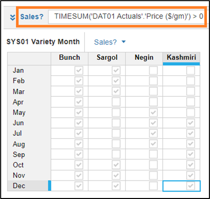
6) We set up another module ‘SYS01 Variety Month’ at the Variety and Month level, and introduce ‘Sales?’ Boolean to decipher the months when sales happened in the past. (Again, notice the use of TIMESUM function, since we are aggregating across the time dimension).

7) For User Story 2, we create a new module ‘INP01 Forecast Price’ that is set at Variety, Month and Year level for future three years only. We use ‘Sales?’ Boolean (from previous step) to set up write access (DCA) to enable the users to input price forecast for only the months the given variety is usually sold in.

8) To conclude User Story 2, we set up a page for the user to select a variety and input price forecast for future years (‘INP01 Forecast Price’), while referring to the historical prices for past years (‘DAT01 Actuals’).

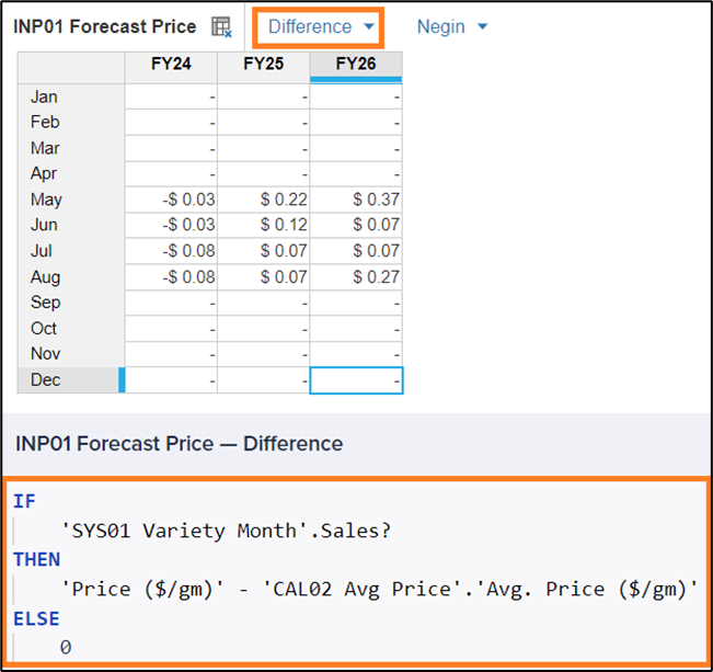
9) For User Story 3, we create a line item ‘Difference’ in ‘INP01 Forecast Price’ to store the difference between Price and Avg. Price. Notice the use of ‘Sales?’ Boolean in the formula.

10) To conclude User Story 3, we set up conditional formatting on the line-item Price in the module ‘INP01 Forecast Price’ as shown below.

Now, user should be able to easily identify cells (through red color) that have Forecast Price set below the 3-yr Average Price.

Conclusion

With the current set of requirements, we learnt about one application of TIMESUM function. The function was used in a situation where Time dimension had to be ditched completely so that the given measure could be summed up across all the available time periods (past three years).

That said, the function could also be used in situations where we need aggregation across a limited window of the Time dimension. For example, calculating sum across just two time periods — FY22 and FY23. In fact, we could use the function to extract value off a specific time period as well.

Last but not the least, the function is not limited to just one aggregation method SUM. It could also be used for other aggregation methods such as average, minimum, maximum, etc.